
지난 포스트에서 볼린저 밴드, 켈트너 채널, 슈퍼트렌드를 각각 소개했고, 슈퍼트렌드가 추세추종 시스템으로서 압도적인 성과를 보였습니다. 이번 글에서는 슈퍼트렌드의 청산 방식을 개선해서 수익을 더 잘 보존하는 전략을 다룹니다.
문제: 슈퍼트렌드 전환 청산의 한계
슈퍼트렌드 설명 포스트에서의 기본 매매 방식은 "상승 전환 → 매수, 하락 전환 → 매도"였습니다. 문제는 하락 전환이 너무 늦게 온다는 것입니다.
슈퍼트렌드는 밴드가 한 방향으로만 이동하기 때문에, 가격이 꽤 많이 떨어져야 비로소 전환이 발생합니다. 큰 상승을 잡아도, 정점에서 상당 부분을 반납한 뒤에야 청산됩니다.
ATR은 이런 상황에 적합합니다. 진입 후 최고가에서 N×ATR만큼 떨어지면 청산하는 ATR 트레일링 스톱은, 슈퍼트렌드 전환보다 더 빠르게 수익을 보존할 수 있습니다.
전략 설계
진입: 슈퍼트렌드 상승 전환 (하락 → 상승, 빨강 → 초록). 22편과 동일합니다.
청산: 진입 후 최고가 - N×ATR(14). 최고가는 진입 이후 기록된 고가 중 최댓값으로, 가격이 올라갈수록 스톱도 따라 올라갑니다. 가격이 이 스톱 아래로 내려오면 청산합니다.
트레일링 스톱 = 진입 후 최고가 - N × ATR(14)
종가 < 트레일링 스톱  →  청산
슈퍼트렌드 전환 청산(베이스라인)과 비교하기 위해 ATR 배수 N = 2, 3, 4를 테스트합니다.


백테스트 조건
| 항목 | 설정 |
|---|---|
| 종목 | BTC/USDT (Binance Spot) |
| 기간 | 2018.01.01 ~ 2025.12.31 |
| 타임프레임 | 일봉 (1D) |
| 슈퍼트렌드 | ATR 14, ×2.0 |
| 진입 | 슈퍼트렌드 상승 전환 |
| 청산 | ST 전환 (베이스라인) / ATR 트레일링 ×2 / ×3 / ×4 (비교) |
| 초기 자본 | $10,000 |
| 수수료 / 슬리피지 | 미적용 |
슈퍼트렌드 ×2.0을 사용합니다. 지난 포스트에서 ×2.0이 가장 민감하게 진입 신호를 잡았고, 청산 개선의 여지가 가장 큰 배수입니다.
코드 구현
import pandas as pd
import numpy as np
import mplfinance as mpf
import matplotlib.pyplot as plt

# ===== 변경 가능한 설정 =====
DATA_FILE = "BTCUSDT_1d.csv"

# 슈퍼트렌드 (진입용)
ST_PERIOD = 14              # ATR 기간. 짧을수록 민감, 길수록 둔감
ST_MULT = 2.0               # ATR 배수. 작을수록 진입 빈번, 클수록 진입 보수적
                            # 22편에서 ×2.0, ×3.0, ×4.0을 비교했음

# ATR 트레일링 스톱 (청산용)
ATR_TRAIL_MULTS = [2.0, 3.0, 4.0]
                            # 청산 배수. 작을수록 빠르게 청산(수익 보존),
                            # 클수록 여유 있게 청산(큰 추세 유지)
                            # 진입용 ST_MULT와 독립적으로 조절 가능

INITIAL_CAPITAL = 10000     # 초기 자본
ZOOM_DAYS = 180             # 차트 확대 구간 (최근 N일)
# ============================

# 데이터 로드
df = pd.read_csv(DATA_FILE, index_col="timestamp", parse_dates=True)

# --- ATR ---
high_low = df["high"] - df["low"]
high_close = (df["high"] - df["close"].shift(1)).abs()
low_close = (df["low"] - df["close"].shift(1)).abs()
tr = pd.concat([high_low, high_close, low_close], axis=1).max(axis=1)
df["atr"] = tr.rolling(window=ST_PERIOD).mean()

# --- 슈퍼트렌드 ---
def calc_supertrend(df, period, multiplier):
    hl2 = (df["high"] + df["low"]) / 2
    atr = df["atr"]
    upper_basic = hl2 + multiplier * atr
    lower_basic = hl2 - multiplier * atr
    upper_band = upper_basic.copy()
    lower_band = lower_basic.copy()
    supertrend = pd.Series(index=df.index, dtype=float)
    direction = pd.Series(index=df.index, dtype=int)
    for i in range(period, len(df)):
        if pd.isna(upper_basic.iloc[i]):
            continue
        if i > period and not pd.isna(upper_band.iloc[i - 1]):
            if upper_basic.iloc[i] < upper_band.iloc[i - 1] or df["close"].iloc[i - 1] > upper_band.iloc[i - 1]:
                upper_band.iloc[i] = upper_basic.iloc[i]
            else:
                upper_band.iloc[i] = upper_band.iloc[i - 1]
        if i > period and not pd.isna(lower_band.iloc[i - 1]):
            if lower_basic.iloc[i] > lower_band.iloc[i - 1] or df["close"].iloc[i - 1] < lower_band.iloc[i - 1]:
                lower_band.iloc[i] = lower_basic.iloc[i]
            else:
                lower_band.iloc[i] = lower_band.iloc[i - 1]
        if i == period:
            direction.iloc[i] = 1 if df["close"].iloc[i] > upper_band.iloc[i] else -1
        else:
            prev_dir = direction.iloc[i - 1]
            if prev_dir == -1 and df["close"].iloc[i] > upper_band.iloc[i]:
                direction.iloc[i] = 1
            elif prev_dir == 1 and df["close"].iloc[i] < lower_band.iloc[i]:
                direction.iloc[i] = -1
            else:
                direction.iloc[i] = prev_dir
        supertrend.iloc[i] = lower_band.iloc[i] if direction.iloc[i] == 1 else upper_band.iloc[i]
    return supertrend, direction

st, direction = calc_supertrend(df, ST_PERIOD, ST_MULT)
df["st"] = st
df["st_dir"] = direction
df["st_up"] = df["st"].where(df["st_dir"] == 1, np.nan)
df["st_down"] = df["st"].where(df["st_dir"] == -1, np.nan)

# --- 백테스트: ATR 트레일링 스톱 ---
def run_backtest(df, atr_trail_mult, initial_capital):
    capital = initial_capital
    holdings = 0
    buy_price = 0
    in_position = False
    highest = 0
    trades = []
    equity = []

    for i in range(1, len(df)):
        close = df["close"].iloc[i]
        high = df["high"].iloc[i]
        atr = df["atr"].iloc[i]
        d = df["st_dir"].iloc[i]
        d_prev = df["st_dir"].iloc[i - 1]

        if in_position:
            highest = max(highest, high)

        if not in_position:
            # 슈퍼트렌드 상승 전환 → 진입
            if not pd.isna(d) and not pd.isna(d_prev) and d == 1 and d_prev == -1:
                buy_price = close
                holdings = capital / buy_price
                capital = 0
                in_position = True
                highest = high
        else:
            # ATR 트레일링 스톱 → 청산
            if not pd.isna(atr):
                stop = highest - atr_trail_mult * atr
                if close < stop:
                    capital = holdings * close
                    pnl = (close - buy_price) / buy_price * 100
                    trades.append({"pnl_pct": round(pnl, 2)})
                    holdings = 0
                    in_position = False

        equity.append(capital + holdings * close)

    if in_position:
        last_price = df["close"].iloc[-1]
        capital = holdings * last_price
        pnl = (last_price - buy_price) / buy_price * 100
        trades.append({"pnl_pct": round(pnl, 2)})

    eq = pd.Series(equity)
    peak = eq.cummax()
    mdd = ((eq - peak) / peak * 100).min()

    return capital, trades, mdd, equity

# --- 베이스라인: ST 전환 청산 ---
def run_st_only(df, initial_capital):
    capital = initial_capital
    holdings = 0
    buy_price = 0
    in_position = False
    trades = []
    equity = []

    for i in range(1, len(df)):
        close = df["close"].iloc[i]
        d = df["st_dir"].iloc[i]
        d_prev = df["st_dir"].iloc[i - 1]

        if not in_position:
            if not pd.isna(d) and not pd.isna(d_prev) and d == 1 and d_prev == -1:
                buy_price = close
                holdings = capital / buy_price
                capital = 0
                in_position = True
        else:
            if not pd.isna(d) and not pd.isna(d_prev) and d == -1 and d_prev == 1:
                capital = holdings * close
                pnl = (close - buy_price) / buy_price * 100
                trades.append({"pnl_pct": round(pnl, 2)})
                holdings = 0
                in_position = False

        equity.append(capital + holdings * close)

    if in_position:
        capital = holdings * df["close"].iloc[-1]
        pnl = (df["close"].iloc[-1] - buy_price) / buy_price * 100
        trades.append({"pnl_pct": round(pnl, 2)})

    eq = pd.Series(equity)
    mdd = ((eq - eq.cummax()) / eq.cummax() * 100).min()
    return capital, trades, mdd, equity

# --- 바이앤홀드 ---
first_price = df["close"].dropna().iloc[0]
last_price = df["close"].dropna().iloc[-1]
bnh_return = (last_price - first_price) / first_price * 100
bnh_capital = INITIAL_CAPITAL * (1 + bnh_return / 100)

# --- 실행 ---
print("=" * 95)
print(f"SuperTrend (ATR {ST_PERIOD}, x{ST_MULT}) + ATR Trailing Stop")
print(f"Entry: ST bullish flip / Exit: Highest - N x ATR")
print(f"Data: {df.index[0].strftime('%Y-%m-%d')} ~ {df.index[-1].strftime('%Y-%m-%d')}")
print("=" * 95)
print(f"  {'Exit':<25} {'Capital':>10} {'Return':>10} {'MDD':>8} {'Trades':>7} {'Win':>5} {'Lose':>5} {'WinRate':>8} {'AvgW':>8} {'AvgL':>8}")
print("-" * 95)

cap0, trades0, mdd0, eq0 = run_st_only(df, INITIAL_CAPITAL)
ret0 = (cap0 - INITIAL_CAPITAL) / INITIAL_CAPITAL * 100
w0 = len([t for t in trades0 if t["pnl_pct"] > 0])
l0 = len([t for t in trades0 if t["pnl_pct"] <= 0])
wr0 = w0 / len(trades0) * 100 if trades0 else 0
avgw0 = np.mean([t["pnl_pct"] for t in trades0 if t["pnl_pct"] > 0]) if w0 > 0 else 0
avgl0 = np.mean([t["pnl_pct"] for t in trades0 if t["pnl_pct"] <= 0]) if l0 > 0 else 0
print(f"  {'ST Flip (baseline)':<25} ${cap0:>9,.0f} {ret0:>+9.2f}% {mdd0:>+7.2f}% {len(trades0):>6}  {w0:>5} {l0:>5} {wr0:>7.1f}% {avgw0:>+7.1f}% {avgl0:>+7.1f}%")
print()

results = {}
for trail_mult in ATR_TRAIL_MULTS:
    cap, trades, mdd, eq = run_backtest(df, trail_mult, INITIAL_CAPITAL)
    ret = (cap - INITIAL_CAPITAL) / INITIAL_CAPITAL * 100
    w = len([t for t in trades if t["pnl_pct"] > 0])
    l = len([t for t in trades if t["pnl_pct"] <= 0])
    wr = w / len(trades) * 100 if trades else 0
    avgw = np.mean([t["pnl_pct"] for t in trades if t["pnl_pct"] > 0]) if w > 0 else 0
    avgl = np.mean([t["pnl_pct"] for t in trades if t["pnl_pct"] <= 0]) if l > 0 else 0
    print(f"  {'ATR Trail x' + str(trail_mult):<25} ${cap:>9,.0f} {ret:>+9.2f}% {mdd:>+7.2f}% {len(trades):>6}  {w:>5} {l:>5} {wr:>7.1f}% {avgw:>+7.1f}% {avgl:>+7.1f}%")
    results[trail_mult] = eq

print("-" * 95)
print(f"  {'B&H':<25} ${bnh_capital:>9,.0f} {bnh_return:>+9.2f}%")
print("=" * 95)

# --- 에쿼티 커브 비교 ---
fig, ax = plt.subplots(figsize=(14, 6))
ax.plot(eq0, label=f"ST x{ST_MULT} Flip Exit (baseline)", alpha=0.7)
for trail_mult in ATR_TRAIL_MULTS:
    ax.plot(results[trail_mult], label=f"ST x{ST_MULT} + ATR Trail x{trail_mult}", alpha=0.8)
ax.set_title(f"Equity Curve - SuperTrend x{ST_MULT} Exit Strategies")
ax.set_ylabel("Equity ($)")
ax.legend()
ax.grid(True, alpha=0.3)
plt.tight_layout()

# --- 차트: 슈퍼트렌드 (상승장) ---
df_bull = df.loc["2020-10-01":"2021-04-30"].copy()
ap_bull = [
    mpf.make_addplot(df_bull["st_up"], color="#43A047", width=1.5),
    mpf.make_addplot(df_bull["st_down"], color="#E53935", width=1.5),
]
fig2, axes2 = mpf.plot(df_bull, type="candle", style="charles",
    title=f"BTC/USDT  SuperTrend (x{ST_MULT}) + ATR Trail (2020.10 ~ 2021.04)",
    volume=False, figsize=(14, 8),
    addplot=ap_bull, returnfig=True)

# --- 차트: 최근 구간 ---
df_zoom = df.tail(ZOOM_DAYS).copy()
ap_zoom = [
    mpf.make_addplot(df_zoom["st_up"], color="#43A047", width=1.5),
    mpf.make_addplot(df_zoom["st_down"], color="#E53935", width=1.5),
]
fig3, axes3 = mpf.plot(df_zoom, type="candle", style="charles",
    title=f"BTC/USDT  SuperTrend (x{ST_MULT}) + ATR Trail (Last {ZOOM_DAYS}D)",
    volume=False, figsize=(14, 8),
    addplot=ap_zoom, returnfig=True)

plt.show()
테스트 포인트
코드 상단의 설정 블록에서 다음 변수들을 조절할 수 있습니다.
ST_PERIOD (기본 14) — 슈퍼트렌드에 사용할 ATR 기간. 짧게 하면(예: 7, 10) 최근 변동성에 민감하게 반응하고, 길게 하면(예: 20, 30) 더 장기적인 변동성을 반영합니다. 이 값은 진입과 청산 양쪽에 영향을 줍니다.
ST_MULT (기본 2.0) — 슈퍼트렌드 ATR 배수. 진입 감도를 결정합니다. 22편에서 ×2.0(민감), ×3.0(기본), ×4.0(둔감)을 비교했습니다. 작을수록 진입 빈도가 높아지고, 클수록 확실한 추세 전환에서만 진입합니다.
ATR_TRAIL_MULTS (기본 [2.0, 3.0, 4.0]) — ATR 트레일링 스톱 배수. 청산 속도를 결정합니다. 이 값은 ST_MULT와 독립적으로 조절할 수 있습니다. 작을수록(×2.0) 빠르게 수익을 확정하지만 조기 청산 위험이 있고, 클수록(×4.0~5.0) 큰 추세를 오래 타지만 정점에서 많이 반납합니다. [1.5, 2.0, 2.5, 3.0, 3.5, 4.0, 5.0] 같이 세밀하게 비교해볼 수 있습니다.
INITIAL_CAPITAL (기본 10000) — 수익률과 MDD는 비율이라 이 값에 영향받지 않지만, 에쿼티 커브의 Y축 스케일이 바뀝니다.
ZOOM_DAYS (기본 180) — 차트 마지막 N일 확대 구간. 더 넓게 보려면 365, 좁게 보려면 90으로 조절하면 됩니다.
결과 분석
===============================================================================================
SuperTrend (ATR 14, x2.0) + ATR Trailing Stop
Entry: ST bullish flip / Exit: Highest - N x ATR
Data: 2018-01-01 ~ 2025-12-31
===============================================================================================
  Exit                         Capital     Return      MDD  Trades   Win  Lose  WinRate     AvgW     AvgL
-----------------------------------------------------------------------------------------------
  ST Flip (baseline)          $  106,919   +969.19%  -53.76%     62     26    36    41.9%   +24.4%    -7.7%

  ATR Trail x2.0             $   83,845   +738.45%  -46.48%     62     27    35    43.5%   +19.1%    -6.2%
  ATR Trail x3.0             $  232,558  +2225.58%  -44.45%     52     24    28    46.2%   +29.1%    -7.6%
  ATR Trail x4.0             $  152,113  +1421.13%  -67.19%     40     18    22    45.0%   +46.8%   -10.8%
-----------------------------------------------------------------------------------------------
  B&H                        $   65,507   +555.07%
===============================================================================================| 청산 | 수익률 | MDD | 거래 | 승률 | 평균 수익 | 평균 손실 |
|---|---|---|---|---|---|---|
| ST 전환 (baseline) | +969% | -53.76% | 62 | 41.9% | +24.4% | -7.7% |
| ATR Trail ×2.0 | +738% | -46.48% | 62 | 43.5% | +19.1% | -6.2% |
| ATR Trail ×3.0 | +2225% | -44.45% | 52 | 46.2% | +29.1% | -7.6% |
| ATR Trail ×4.0 | +1421% | -67.19% | 40 | 45.0% | +46.8% | -10.8% |
ATR Trail ×3.0이 베이스라인 대비 모든 지표에서 개선됐습니다.
수익률: +969% → +2225%. 2배 이상 증가했습니다. 슈퍼트렌드 전환 청산은 정점에서 많이 반납한 뒤에야 빠져나오는데, ATR 트레일링은 정점 근처에서 더 빠르게 수익을 확정합니다. 같은 진입 신호에서 출발해도 청산 타이밍 하나로 이만큼 차이가 납니다.
MDD: -53.76% → -44.45%. 약 9%p 개선. 에쿼티 커브 차트에서 ATR Trail ×3.0(초록)이 다른 전략들보다 일관되게 높은 위치를 유지하는 것이 보입니다.
승률: 41.9% → 46.2%. 소폭이지만 일관된 개선. 빠른 청산으로 작은 수익이라도 확정하는 거래가 늘었습니다.
거래 수: 62 → 52. 10회 줄었습니다. ATR Trail이 ST 전환보다 먼저 트리거되면서, 일부 경우 다음 ST 상승 전환까지 기다리는 구간이 달라진 결과입니다.
평균 수익/손실 비율: 베이스라인의 AvgW/AvgL = 24.4/7.7 = 3.17:1, ATR Trail ×3.0 = 29.1/7.6 = 3.83:1. 평균 손실은 거의 같은데(-7.7% vs -7.6%), 평균 수익이 +24% → +29%로 올랐습니다. 수익 거래에서 더 많이 가져가고, 손실 거래는 비슷한 수준으로 통제한 것입니다.
×2.0과 ×4.0은 왜 ×3.0보다 나쁜가? ×2.0은 너무 빠르게 청산해서 큰 추세를 중간에 끊습니다(AvgW +19%, 거래 62회). ×4.0은 너무 느려서 수익 반납이 커집니다(MDD -67%). ×3.0이 "추세를 충분히 타되, 반전 시 빠르게 빠지는" 균형점에 있습니다.
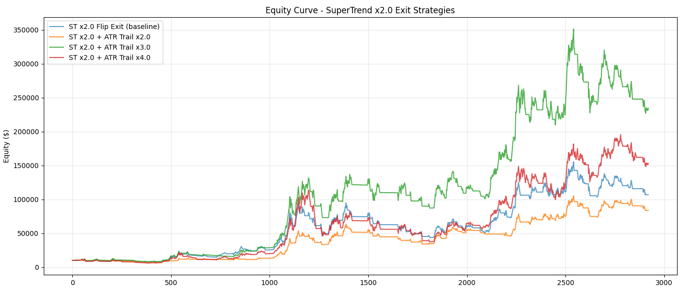
에쿼티 커브에서 ATR Trail ×3.0(초록)이 2024년 이후 구간에서 특히 다른 전략들과 격차를 벌리는 것이 보입니다. 큰 상승을 잡은 뒤 정점 근처에서 빠져나와 수익을 보존한 결과입니다.
정리
슈퍼트렌드 진입 + ATR 트레일링 스톱 청산은 진입 시스템과 청산 시스템을 분리한 전략입니다. 22편에서 슈퍼트렌드가 진입과 청산을 모두 담당했지만, 청산만 ATR 트레일링으로 교체하는 것만으로 수익률이 2배 이상, MDD는 9%p 개선됐습니다.
핵심 교훈은 "좋은 진입만큼 좋은 청산이 중요하다"는 것입니다. 같은 진입 신호라도 청산 방식에 따라 결과가 극적으로 달라집니다. 진입은 슈퍼트렌드 같은 추세 전환 감지기가, 청산은 ATR 같은 변동성 기반 트레일링 스톱이 각자의 역할에 더 적합합니다.
본 포스팅은 지표의 원리와 백테스트 과정을 정리한 기술 블로그이며, 특정 자산의 매매를 권유하지 않습니다.
백테스트 결과는 과거 데이터 기반이며 실제 수익을 보장하지 않습니다. 모든 투자의 책임은 본인에게 있습니다.
'Development > Indicator Lab' 카테고리의 다른 글
| NNFX 프레임워크 소개 (1) | 2026.04.02 |
|---|---|
| TTM Squeeze (0) | 2026.04.01 |
| 슈퍼트렌드 (SuperTrend) (0) | 2026.03.30 |
| 켈트너 채널 (Keltner Channel) (0) | 2026.03.29 |
| 볼린저 밴드 (Bollinger Bands) (0) | 2026.03.28 |